What is MiSa.C?

The Minimal Sampling Classifier (MiSa.C) is an innovative web service for the classification of remote sensing raster image data, which allows the classification of complex surfaces in space and time. It originates from Habitat Sampler (HaSa), a command line tool developed by Dr. Carsten Neumann at the Helmholtz Center Potsdam German Research Center for Geosciences GFZ in Potsdam, Germany.

MiSa.C’s key advantages are:

• MiSa.C requires only one reference point per class and eliminates the need for extensive ground truth data by automatically generating training points.

• The tool offers a choice of two robust machine learning classification algorithms:

  • Random forest

  • Support vector machine

• Users have complete control over the output classification by an interactive setting of classification thresholds in the easy-to-use graphical interface, incorporating expert knowledge rather than relying on a black box algorithm.

• Users can adjust input parameters throughout the classification process, allowing them to observe the output and proceed only if they are satisfied with the results.

• MiSa.C provides easy output of result maps and images.

• The tool supports input raster imagery from various sensors and resolutions.

• Optional: Users have the option of retrieving preprocessed, atmospheric-corrected Sentinel-2 time series data directly from the interface as input data.

How does it work?

The MiSa.C interface guides the user step-by-step through the classification process, with the following key steps:

• Step 0: Create a workspace by giving it a unique name and an optional description.

• Step 1: Input representative reference data by uploading a shapefile or table data.

• Step 2: Input layer image stack by using your own data stack or by accessing Sentinel-2 data from the internal download service.

• Step 3: Run the interactive, step-by-step classification algorithm that outputs results for one class at a time. Users can repeat the classification process for a single class until they are satisfied with the results before moving on to the next class.

• Results: View the results in the map view within MiSa.C or download the results for further analysis using external tools.

Getting to know the MiSa.C classification process

This tutorial will guide the user through the classification process in MiSa.C and provide explanations for each step. In addition, solutions are offered to help the user achieve a satisfactory classification result.

Step 0: Creation of a workspace

Before starting a classification, a new workspace must be created. In this workspace, the project or location can be given a meaningful name and optionally a description. Each user can have up to 15 workspaces.

Note: If a workspace with the same name already exists, it cannot be selected again.

Step 1: Input of reference data

Once the user has created a workspace, representative reference data can be uploaded. MiSa.C offers two options for this: uploading an ESRI shapefile in .zip format or uploading data from a table in .txt format. When uploading an ESRI shapefile, the locations of the reference data resp. reference points (one per class) are uploaded and class information is retrieved directly from the data at the specified point locations. It is important to note that all reference points must be within the area of interest being analysed. If the reference points are dispersed and not directly in the area of interest, users can also upload the spectral information using a reference data table. Finally, the number of reference data values per class must exactly match the number of layers (dates x spectral bands) of the raster stack.

Option A) Shapefile

The user provides the representative reference data as a shapefile, with all points located within the analysed area of interest.

Representative reference data stored in a shapefile must contain point data, with one point per class. Each point in the reference data shapefile also needs to have the corresponding class name stored in a dedicated column with the name “class”. A class name should not contain any special character or white spaces. Optionally, after uploading the reference data, classes that are not to be used for classification can be deselected.

The required formats for a shapefile from a local directory are:

• *.dbf

• *.prj

• *.shp

• *.shx

Note: Currently, MiSa.C supports a maximum of 20 classes for one classification run. The shapefile must also have a geospatial projection information. MiSa.C will automatically adjust the projection if it does not match the projection of the input raster data.

Option B) Table file

If the user has representative reference data available that is not located within the area of interest, but contains the same band information.

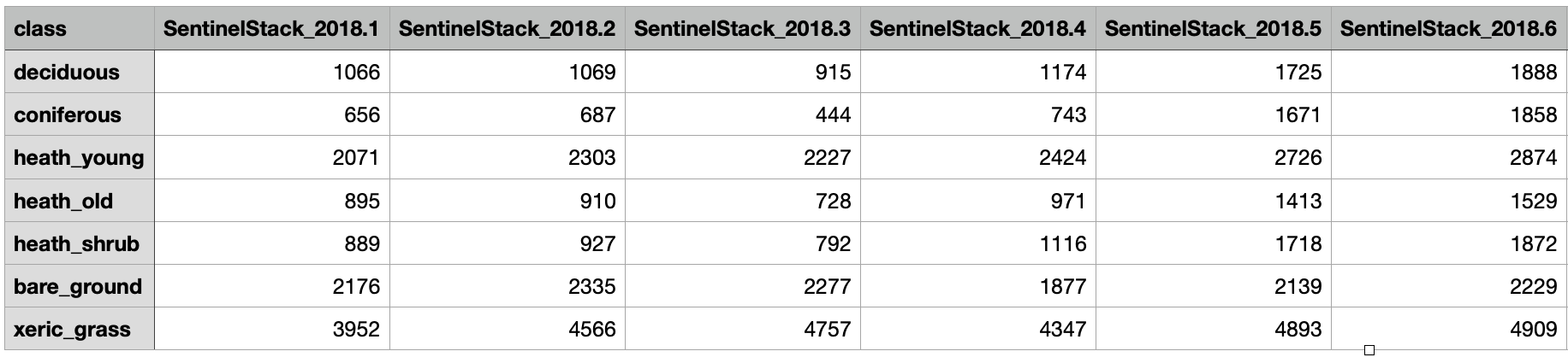
Representative reference data that is not located in the area of interest can be uploaded as a table in .txt format. The first column should contain the class names and the first row should contain the corresponding band names. The reference data table should be formatted as shown in the figure below.

MiSa.C will validate the input of the image layer stack to check if the number of reference data values per class matches the exact number of layers (dates x spectral bands) of the raster stack. If the validation fails, the user cannot proceed. This option cannot be used in combination with the download service, as in this case the band information cannot be aligned.

Step 2: Input of an image layer stack

There are two ways of adding an image layer stack. One is the build-in download service which is only available if the representative reference data is in shapefile format. The other one is to upload a local image layer stack.

Note: After uploading an image layer stack it is possible to display the representative reference data table in MiSa.C.

Option A) Upload local image layer stack

Before uploading the actual image layer stack, an additional description file in .json format is required. In the section Load JSON description file - requirements it is described how it should be formatted.

After that a local image layer stack can be uploaded. It’s requirements are also described in the Load a local image layer stack – raster data requirements section.

Option B) Image layer stack via download service

MiSa.C has a built-in download service which provides atmosphere-corrected Sentinel-2 imagery by selecting:

• the desired date range,

• the desired bands,

• the required area of interest either by drawing a bounding box or by using a shapefile in .zip format.

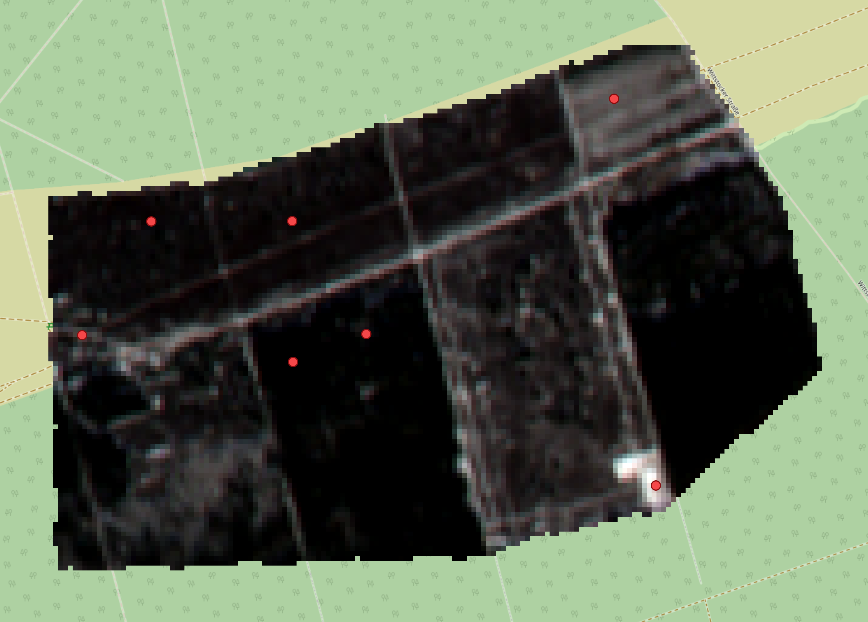
The selected area (bounding box) can cover up to 120km². In a first step, the available dates for the selected period are displayed. From this list between 3 and 12 dates can be selected for classification. After agreeing to the terms and conditions the data will be downloaded. Once the image layer stack is loaded into MiSa.C and a shapefile was used for the representative reference data, the user should see both the previously uploaded reference points and the satellite imagery. This should look similar to the figure below:

Check image layer stack for cloud cover

If the built-in download service is used, the user needs to check the image layer stack for possible cloud coverage, otherwise the surface classification will be incorrect.

To do this, the user must click on the Add a new RGB layer button. In the newly opened tab, the same date needs to be selected for each RGB component of the stack. After giving the layer a meaningful name and clicking Create, these new layers are automatically displayed at the top of the map and can be checked for cloud cover. If cloud cover is detected, the layer needs to be excluded from the classification (Classification Process). This will be repeated for each date.

Load JSON description file - requirements

To start the upload of the local image layer stack, the user must upload a description file containing the dates of each scene in the raster stack and the band names. This information about dates and bands allows the user to build custom RGB layers on the fly that can be used as a reference during the classification. The description file is uploaded as a .json file following the format below:

{
  "dates": ["YYYY-MM-DD", "YYYY-MM-DD", ...]
  "bands": ["band name 1", "band name 2", ...]
}

There should be a maximum of 12 dates. Optionally, the user can also provide information about NoData values used in the data. Pixels with these values will be excluded from the classification process:

{
  "dates": ["YYYY-MM-DD", "YYYY-MM-DD", ...]
  "bands": ["band name 1", "band name 2", ...]
  "nodata": ["0", ...]
}

A .json template for any custom data stack is available here.

Load a local image layer stack – raster data requirements

To work with MiSa.C, all raster data need to be combined into a single data stack, like shown in the following example:

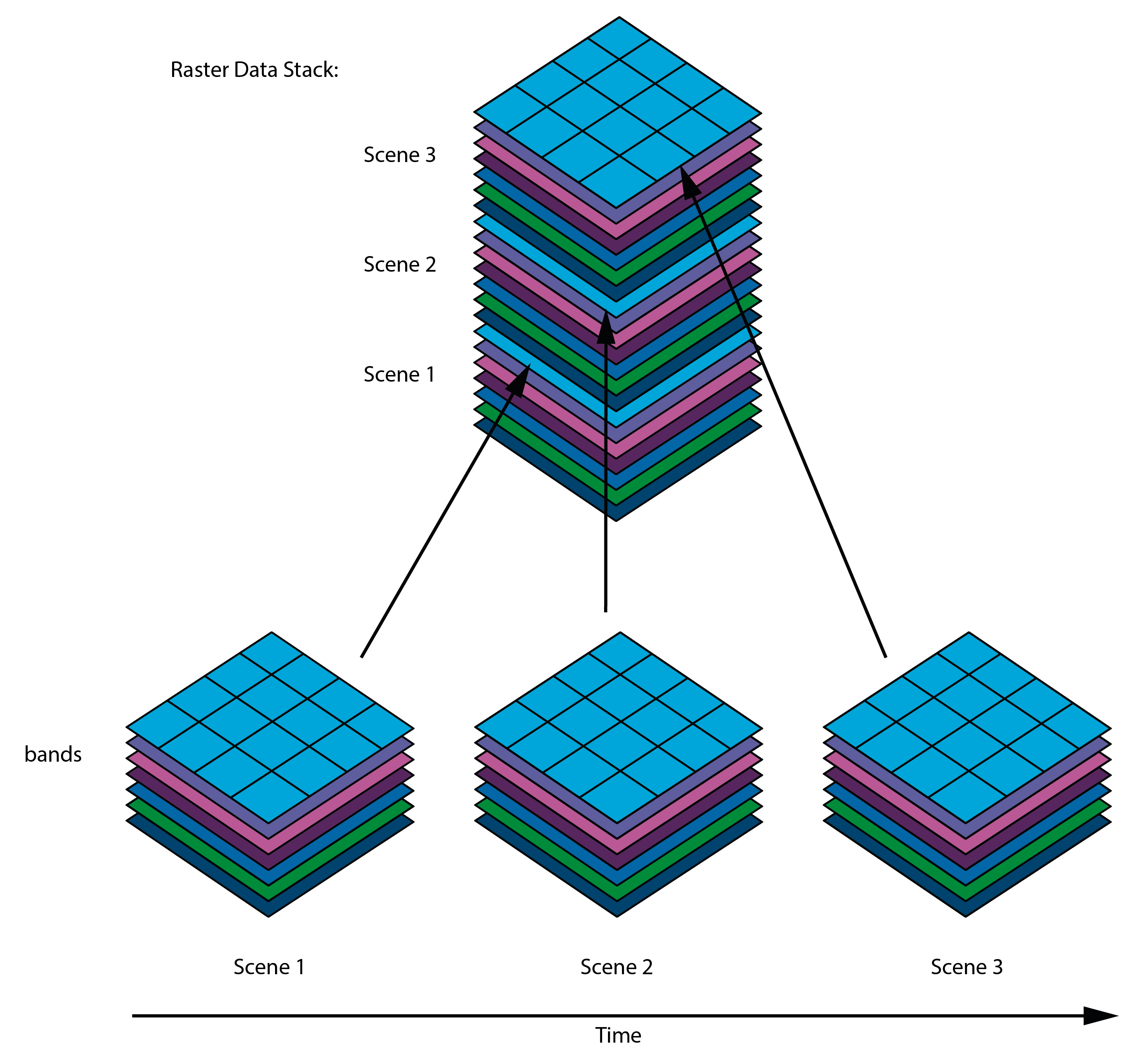
• All layers in the raster data stack must have the same spatial extent.

• All pixels in the raster data stack must have the same spatial resolution and the same projection.

• The Coordinate Reference System (CRS) must be defined in UTM.

• All pixels need to contain meaningful information, the algorithm cannot work properly if some pixels have cloud cover. It is the user’s responsibility to prepare the data accordingly.

• All individual image scenes need to contain precisely the same bands (number of bands and spectral information).

• The layers should be ordered correctly in time, this means the oldest image (1st in time) goes to the bottom and the latest (last in time) to the top.

• The maximum size of an uploaded raster stack must not exceed 250 MB.

• The bit depth of the raster stack must be 32 bit.

Step 3: Surface classification

Understanding MiSa.C

In order to have a better understanding of what MiSa.C does, some background information is given below:

• Sampling: MiSa.C samples and automatically detects pixels with similar spectral properties. The automatic search for training data can either be realised with a regular grid of pixels or by testing random pixels for similarity. Note that the regular grid of samples is faster than random. However, it fails when a lot of NoData values exist, as an increasing number of points fall within these areas. This also happens when more and more pixels are already assigned to a class. Random sampling is slower, but only samples pixels within valid, unclassified pixels. If classification results are not satisfying, the user should try to increase the number of samples and change the sampling distribution.

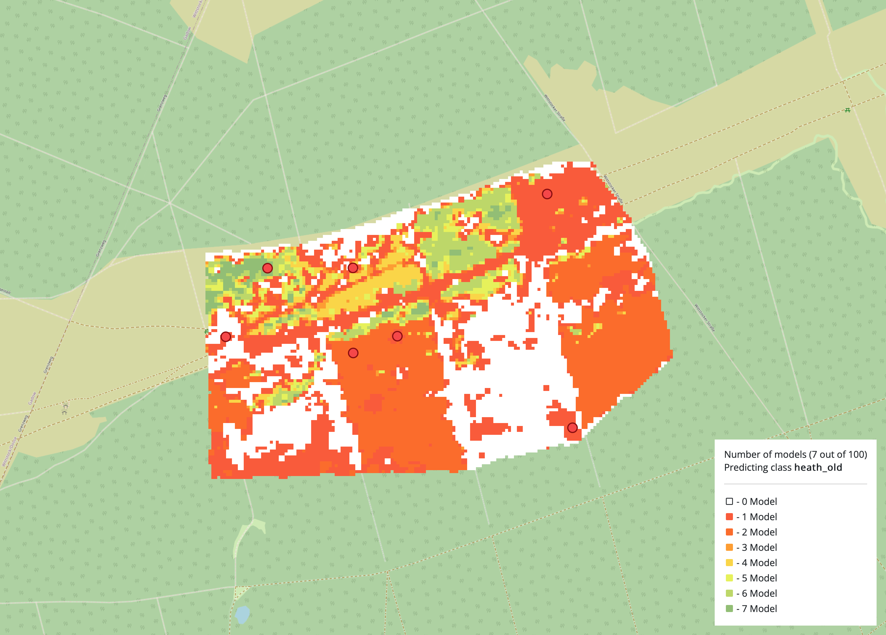
• Modelling: Based on the automatic training point selection, the machine learning algorithm chosen by the user tries to build as many models as specified with the parameter “number of models”. After that those models are tested if they can distinguish one class from all the others by the reference data provided by the user. If that’s the case this particular model is saved. After all models are tested against all classes, the class with the most models is selected. MiSa.C then uses one of those specific models for the selected class to decide whether a pixel of the image data stack belongs to the given class or not. This is done multiple times, referring to the number of models chosen for that class. The results are then displayed on the map. Results in this context are the number of models that can clearly separate one class from the other classes. If the classification result is not satisfying, the user can change the machine learning algorithm used for the classification or increase the number of models.

• Customisation: For each step, MiSa.C displays the number of models that have identified a particular pixel as belonging to a class. The higher the number of models, the higher the probability that the pixel is classified correctly. MiSa.C enables the user to incorporate their expert knowledge to decide for a good threshold for the number of models that classified the pixels correctly. Note that with fewer remaining classes the number of models assigning pixels to a certain class will increase. If the classification result is not satisfying the user should make use of the option to re-sample, either with the same input parameters, or if repeated sampling is not improving the result, with adapted parameter settings.

Classification process

The Start classification button allows the user to start the surface classification process. This opens a tab showing the number of classification steps available, the current step, and the various parameters that can be adjusted for classification. The tab also shows which data has been selected and which bands are being used. This allows the user to check that they have made the right choices.

The adjustable parameters are

• Initial Number of Samples

• Initial Number of Models

and in the Advanced Settings tab

• Band selection: The user can (un-)select certain bands or whole scenes. As default all bands and scenes are selected. If the internal download service was used, it is important at this point to deselect the entire date if clouds were detected during the check (Check image layer stack for cloud cover).

• Machine Learning Algorithm: The options are random forest and support vector machine. As default random forest is selected.

• Sample Type: The options are regular raster, random raster and random matrix. Default is regular_raster. regular raster is fast but uses a regular grid which includes all pixel at every time including nan-values, which makes it a good choice for the beginning of the classification. With ongoing classification more and more pixels are cut out because they are assigned to a class and those pixels get nan-values. In this case random matrix is a better choice. It is slower but only takes account of pixels with values.

• Threshold (0.00-1.00): During the model training phase, the models are trained until their error is less than 0.02 (that means models reach an accuracy of 98%). If the results are not satisfying the user can try to relax this value slightly (e.g., up to 0.05).

• Predictors: In order to ensure randomness in a random forest procedure the number of predictors always needs to be smaller than the number of input bands and needs to be odd. The recommended value is calculated based on the user’s input data. The default should be \(N_{\text{pred.}}=\sqrt{N_{\text{layers}}}\) (if this number is not odd: +1).

• Distance (in m): By default a buffer of the 8 neighbouring pixels of a sample are checked for their similarity to the sample pixel. The distance value relates to the length of the radius from the center of the sample pixel to the center of the diagonal bordering pixel (in m). Precisely: \(\text{buffersize} = \sqrt{\text{pixRes}^{2} + \text{pixRes}^{2}} \cdot 1.05\), whereas pixRes denotes to the spatial resolution of the data. The buffer size should always be equal to or greater than the radius from the center of a pixel to the diagonal neighbour center. The user has the option to increase the buffer size (the value should be increased incrementally, such as \(2.05 \cdot x\) , \(3.05 \cdot x\) , \(4.05 \cdot x\) , …).

There is not a single setting that suits all - a suitable choice of default parameters depends on the data and the aim of the classification. It is also important to note that the choice of machine learning algorithm can also affect the classification results. Different algorithms have different strengths and weaknesses, and some may perform better on certain types of data or for certain classification tasks.

It is recommended to play around with the default values to get a better feeling for the trade-offs between the number of models received (and thus the granularity of the result can be fine-tuned) and the MiSa.C processing time. A good workflow for MiSa.C is to start with small numbers to get a quick impression of the result and to keep the processing time short. If the result is not satisfactory, the numbers should be increased step by step. So it is best to use the default parameters first. If the user is not satisfied with the result and wants to change the parameters, it is possible to click on the Reclassify button and change the values for the class.

Threshold slider

Once the result for the desired class is obtained, the threshold value for pixels to remain in the corresponding class must be interactively set with the slider. The threshold indicates the number of models that have assigned the pixel to a particular class. The user can now do this for all available classes. If not all classes are to be classified, the user can save and finish the process with the End classification, save and show results button.

Results

The result of the classification process is automatically saved in the user’s workspaces, and the result map is displayed with all classes including unclassified pixels as class “other”.

Note: The results, the original image data stack and metadata can be downloaded by reloading the MiSa.C web application. The download button can be found under “workspace management”.

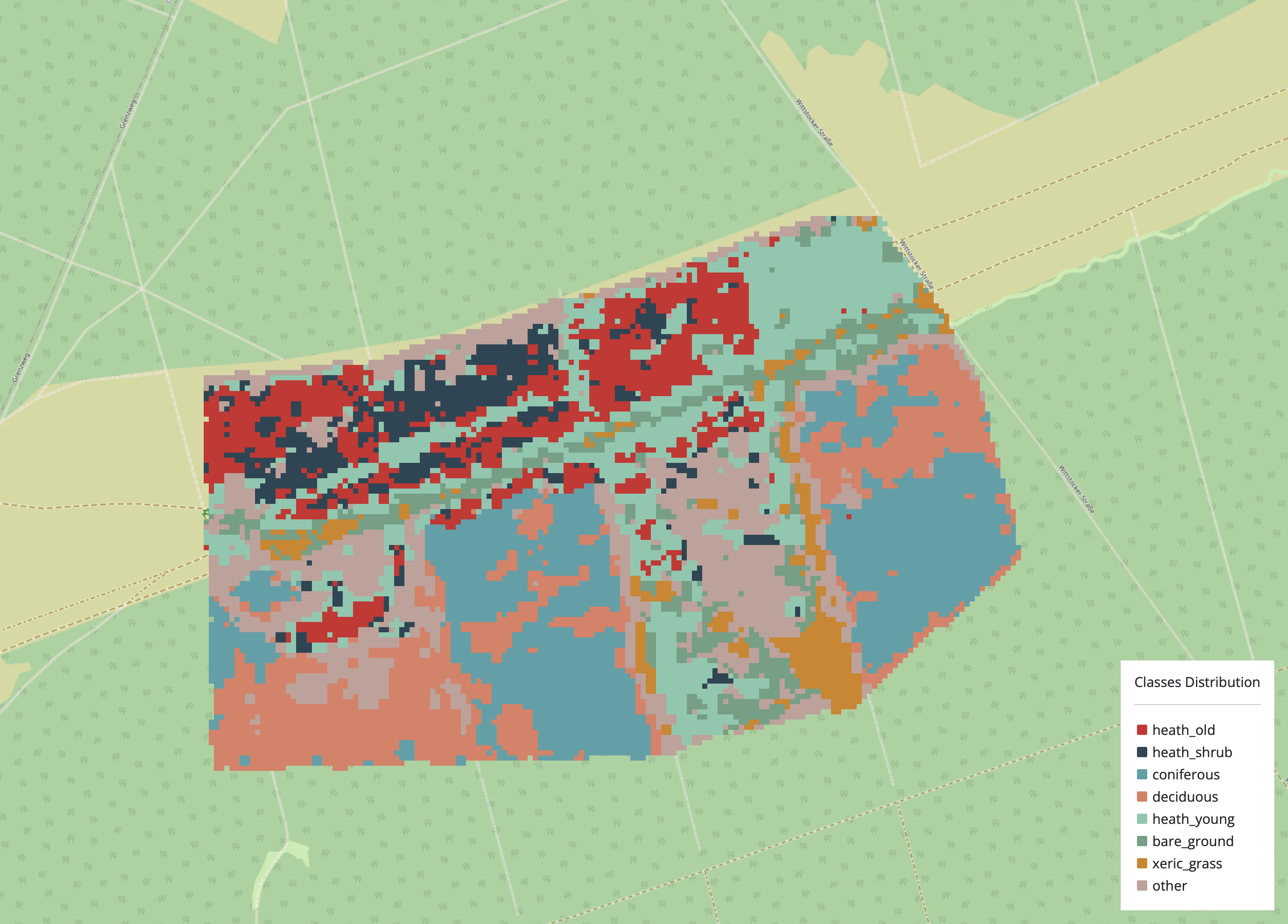
The downloadable results include the result map. It displays all classified and unclassified pixels in a single .tif file, providing a clear overview of all classes in the classification results. This provides an easy way to view the results, use them for further processing, or identify errors or areas that need further attention.

Embedding vector and raster layers into QGIS

Raster data can be embedded into QGIS via a WMS/WMTS connection. To do this, the user must click on the icon for copying the link to the clipboard of the desired class in the layer management on the right side.

The copied link can be used in QGIS under Layer > Add Layer > Add WMS/WMTS-Layer.... Here the user has to click New afterwards, where the copied link can be entered under URL with a conclusive description under Name. After confirming with OK, the option to connect appears, whereupon the available layer can be selected and added to your QGIS project.

Vector data can also be embedded via a new layer in QGIS. In the upper left corner click the icon for the data source manager > vector > source type > Protocol: HTTP(S), cloud, etc. under Protocol > Type choose HTTP, HTTPS, FTP and put the copied link to URI.

Troubleshooting

Classification of surfaces can, under certain circumstances, lead to classification errors. This happens when the number of remaining samples or models is not sufficient to obtain valid models. Another possibility for errors is that the threshold chosen for each class is too low, leaving only a small number of pixels for one of the posterior classes. A tab will pop up telling the user which parameters to change in order to get results. If the problem persists, it is also possible to switch to a different machine learning algorithm, a different sample type, or increase the advanced parameters.

Tutorials

Tutorial 1: classifying a custom image stack with existing reference data.

Tutorial 2: Classifying with the build-in downloader.

Tutorial 3: Classifying a custom image stack with existing tabular reference data.