Tutorial 3: Classifying a custom image stack with existing tabular reference data
In this scenario we show the classification workflow based on provided demo data. Here, we use tabulated data from a 2009 Landsat spectral profile.
The first step is the same as in Tutorial 1: classifying a custom image stack with existing reference data.
Step 1: Upload the reference data as a table
Instead of a shapefile in .zip format, in this tutorial we use reference data of a tabular file in .txt format.
Option B) TableFile

For this purpose we select the second option “TableFile” when uploading the data. In this file is the spectral profile of Landsat from 2009. The nine different ground cover classes used here are deciduous trees, coniferous trees, heather pioneer, bare ground, xeric grass, fresh meadow, heather mature, heather building and heather scrubby.
The following dialogue allows to select the desired classes. In our example, we keep all classes.

In contrast to uploading a shapefile, no reference points are displayed on the map.
Step 2: Input of an image layer stack
If we use a table file as reference data, there is no possibility to use the built-in downloader. So now we use the option
Upload local image layer stack with the .json file as image layer stack description and the image layer stack from
the demo data. This works exactly as in tutorial 1.
After that, we can preview the provided data and upload the stack by clicking the second Add Data button. Our Landsat
time series stack from 2018 consists of data from 3 days with 6 bands each (18 layers in total).

The image stack is then rendered on the map:
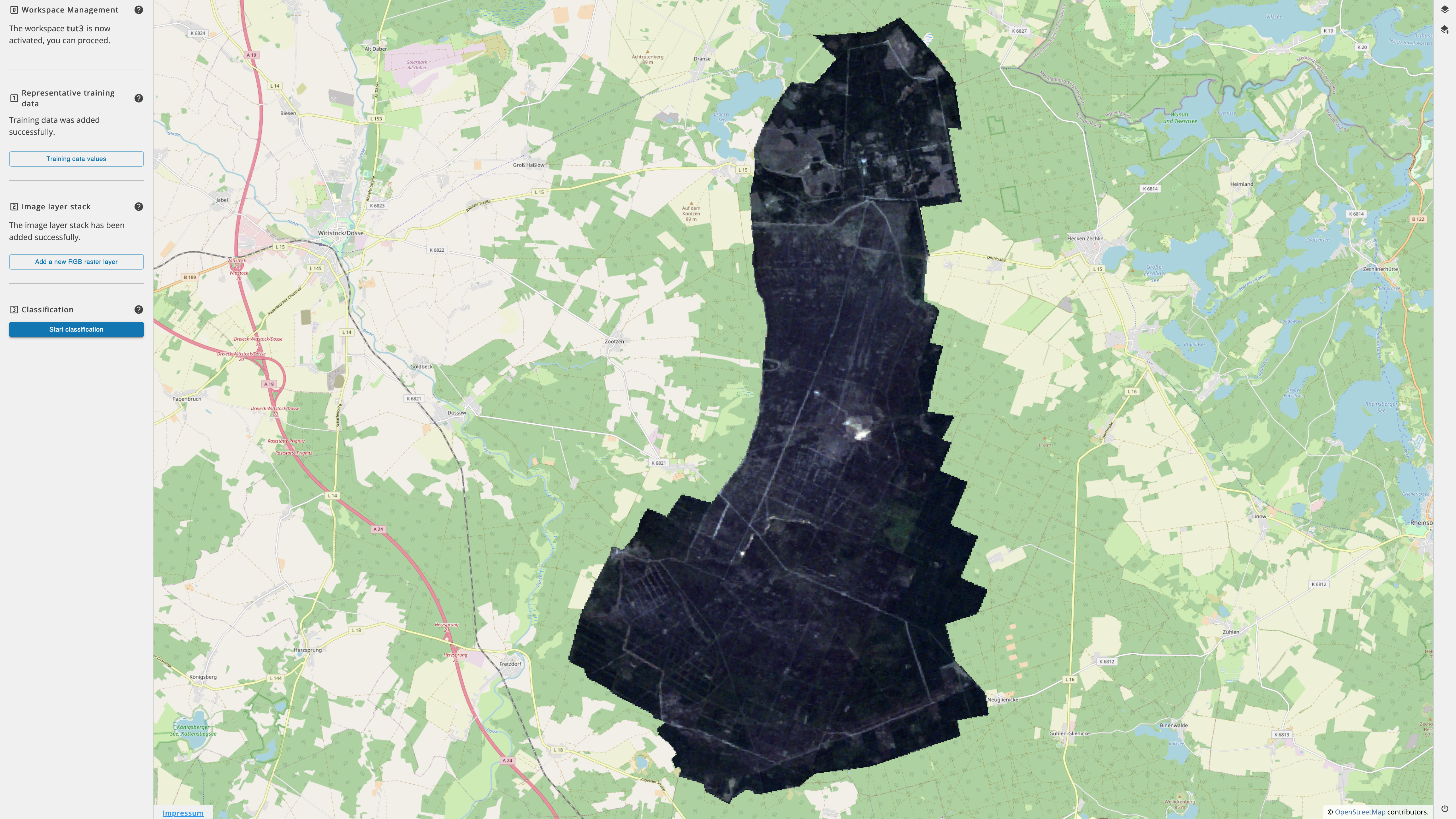
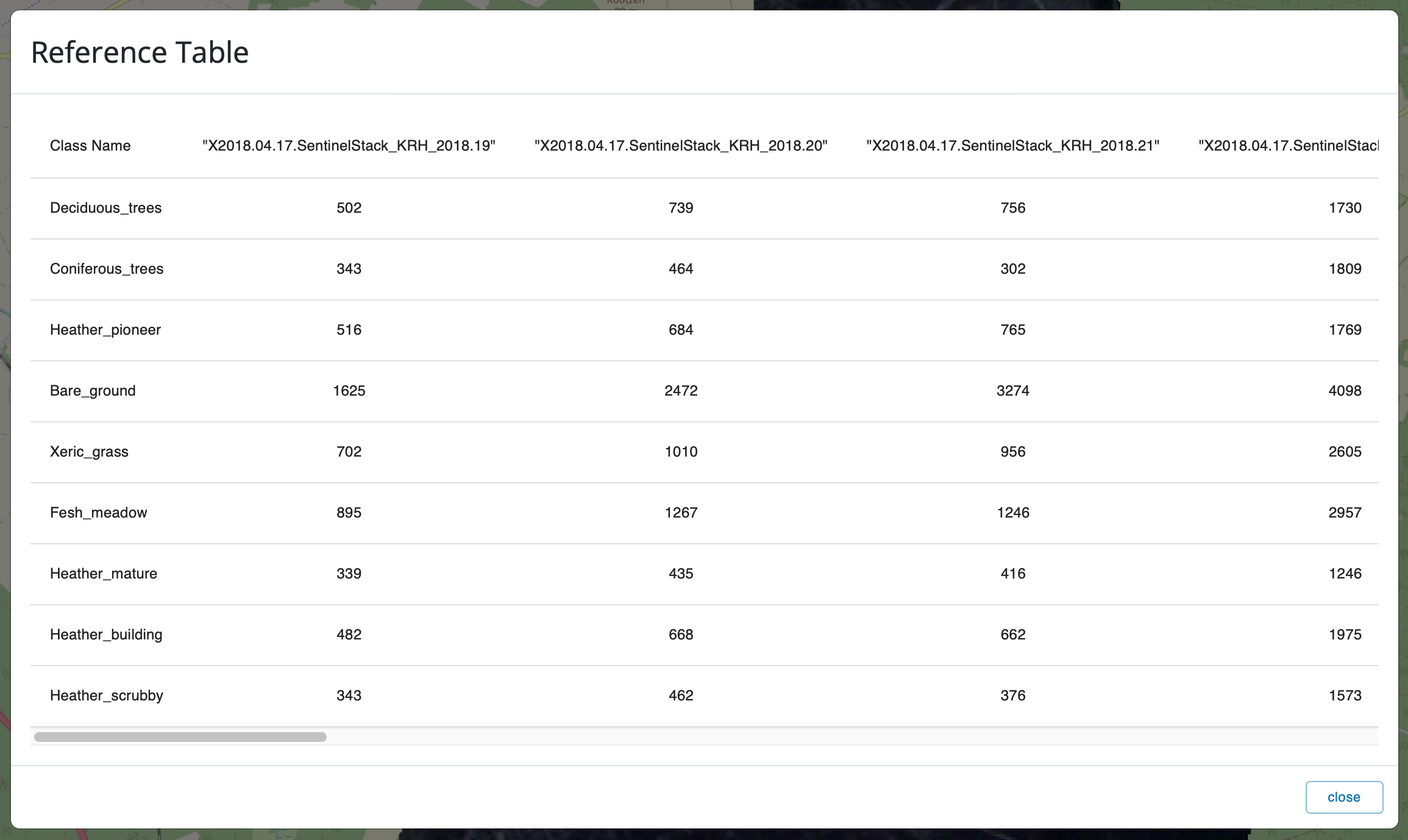
By clicking on the reference data values button on the left, we can also have a look at the reference table and check,
for example, whether everything is correct.
Optional: For better recognizability of the vegetation, we can click here on the button on the left Add a new RGB
raster layer and adjust the band arrangements.
The classification and the rendering of the results is again the same as in tutorial 1.